Bert hamminga Equations Supply and Demand model

A standard teaching version of the model is:

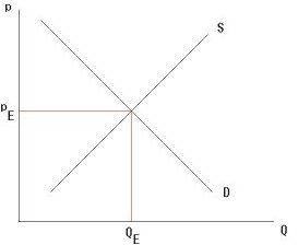
q = S (p)

q = D (p,t)

q is the quantity of supply of some good (say ice) per period in some region
p is price in the period
t is another variable (say temperature)
S is the supply schedule
D is the demand schedule

For simplicity, S en D are often assumed to be linear and

dS / dp > 0 (S is upward sloping to the right)

� D / � t > 0 (Demand rises if, ceteris paribus, t rises)

� D / � p � d S / d p, which makes sure the graphs of the equations have a there is a point of intersection.

From these assumptions it can be proven that dp / dt > 0.

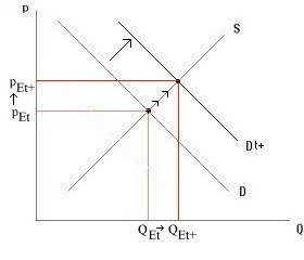This can be illustrated with this graph (right):

High t's (t+) cause an upward shift of D. Since S is assumed to be dependent on p only and rising, the point of intersection should be at a higher p and q when, ceteris paribus, t rises.

Back to: Supply and Demand